This is an R wrapper for agena.ai which provides users capabilities to work with agena.ai using the R environment. Users can create Bayesian network models from scratch or import existing models in R and export to ‘agena.ai’ cloud or local API for calculations.
Note: running calculations requires a valid agena.ai API license (past the initial trial period of the local API).
In the rest of this document, the R environment for agena.ai is referred to as R-Agena.
To install R-Agena from CRAN:
install.packages("agena.ai")R-Agena requires rjson, httr,
Rgraphviz, and openxlsx packages
installed.
To install rjson, httr, and
openxlsx from CRAN:
install.packages('rjson')
install.packages('httr')
install.packages('openxlsx')
To install Rgraphviz from Bioconductor:
if (!require("BiocManager", quietly = TRUE))
    install.packages("BiocManager")

BiocManager::install("Rgraphviz")The Bayesian networks (BNs) in the R environment are represented with
several objects: Node, Network,
DataSet, and Model. These R objects generally
follow their equivalents defined in agena.ai models.
Node objectsThese represent the nodes in a BN. The fields that define a
Node object are as follows:
idMandatory field to create a new Node object. This is the
unique identifier of agena.ai model nodes.
nameName of the node, optional. If not defined, id of the
node will be passed onto the name field too.
descriptionDescription of the node, optional. If not defined, “New Node” will be
assigned to the description field.
typeNode type, it can be:
If it’s not specified when creating a new node, the new node is “Boolean” by default if it’s not a simulation node; and it is “ContinuousInterval” by default if it’s a simulation node.
parentsOther Node objects can be pointed as parents of a
Node object. It is not recommended to modify this field
manually, to add parents to a node, see the function
addParent().
Something to keep in mind: the parent-child relationship information
is stored at Node level in R environment thanks to this
field, as opposed to the separate links field of a
.cmpx/.json file for the agena.ai models. When importing or exporting
.cmpx files you do not need to think about this difference as the cmpx
parser and writer functions handle the correct formats. This difference
allows adding and removing Node objects as parents
simulatedA boolean field to indicate whether the node is a simulation node or not.
distr_typeThe table type of the node, it can be:
statesStates of the node (if not simulated). If states are not specified,
depending on the type, sensible default states are
assigned. Default states for different node types are:
And for a node with the table type (distr_type)
“Expression”, the default expression is: “Normal(0,1000000)”
probabilitiesIf the table type (distr_type) of the node is “Manual”,
the node will have state probabilities, values in its NPT. This field is
a list of these values. The length of the list depends on the node
states and the number of its parents. To see how to set probability
values for a node, see setProbabilities() function.
expressionsIf the table type (distr_type) of the node is
“Expression” or “Partitioned”, the node will have expression(s) instead
of the manually defined NPT values.
expressions field will have a single expression (a single
character string).expressions field will have a list of as many expressions
as the number of parent node states on which the expression is
partitioned.To see how to set the expressions for a node, see
set_expressions() function.
partitionsIf the table type (distr_type) of the node is
“Partitioned”, in addition to the expressions, the node will have the
partitions field. This field is a list of strings, which
are ids of the parent nodes on which the node expression is
partitioned.
variablesThe node variables are called constants on agena.ai Modeller. This field, if specified, sets the constant value for the node observations.
Network objectsThese represent each network in a BN. Networks consist of nodes and
in a BN model there might be more than one network. These networks can
also be linked to each other with the use of input and output nodes. For
such links, see Model$networkLinks field later in this
document.
The fields that define a Network object are as
follows:
idId of the Network. Mandatory field to create a new
network.
nameName of the network, optional. If not specified, id of
the network is passed onto name field as well.
descriptionDescription, optional. If not specified, the string “New Network” is
assigned to description field by default.
nodesA list of Node objects which are in the network. These
Node objects have their own fields which define them as
explained above in this document.
Note that Network objects do not have a
links field unlike the agena.ai models. As explained in
Node$parents section above, this information is stored in
Node objects in the R environment. When importing a .cmpx
model, the information in links field is used to populate
Node$parents fields for each node. Similarly, when
exporting to a .cmpx/.json file, the parent-child information in
Node$parents field is used to create the links
field of the Network field of the .cmpx/.json.
DataSet objectsThese represent the set of observations in a BN. A Model
can have multiple DataSet objects in its
dataSets field. When a new Model is created,
it always comes with a default DataSet object with the
id “Scenario 1” and with blank observations. It is possible
to add more datasets (scenarios) with their ids. Each
DataSet object under a Model can be called a
new “scenario”.
idId of the dataset (scenario).
observationsUnder each dataset (scenario), observations for all the observed
nodes in all the networks of the model (in terms of their states or
values) are listed. If it’s hard evidence, observation for a node will
have a single value with the weight of 1. If a node in the model has a
value in its variable field, this value will be passed onto
the dataset (scenario) with the weight of 1.
resultsThis field is defined only for when a .cmpx model with calculations
is imported. When creating a new BN in the R environment, this field is
not created or filled in. The results field stores the
posterior probability and inference results upon model calculation on
agena.ai Cloud.
Model objectsThese represent the overall BN. A single .cmpx file corresponds to a
singe Model. A BN model can have multiple networks with
their own nodes, links between these networks, and datasets.
idId of the Model, optional. If not specified, the id of
the first Network in the model’s networks
field is used to create a Model$id.
networksA list of all the Network objects that make up the
model. This field is mandatory for creating a new Model
object.
dataSetsOptional field for DataSet objects. When creating a new
Model, it is possible to use predefined scenarios as long
as their DataSet$observations field has matching
ids with the nodes in the model. If none is specified, by
default a new Model object will come with an empty dataset
called “Scenario 1”.
networkLinksIf the Model has multiple networks, it is possible to
have links between these networks, following the agena.ai model
networkLinks format.
To see how to create these links, see add_network_link()
function later in this document.
settingsModel settings for calculations. It includes the
following fields (the values in parantheses are the defaults if settings
are not specified for a model):
Model settings can be provided when creating a new model, if not
provided the model will come with the default settings. Default settings
can be changed later on (with the method
$change_settings()), or model settings can be reset back to
default values (with the method $default_settings()). See
the correct input parameter format for these functions in the following
section. Individual fields in model setting can be adjusted by directly
accessing the field too.
The Node, Network, and Model
objects have their own respective methods to help their definition and
manipulate their fields. The R class methods are used with the
$ sign following an instance of the class. For example,
example_node$add_parent(exampleParentNode)or
example_network$remove_node(exampleNode)or
example_model$create_dataSet(exampleScenario)Node methodsSome Node fields can be modified with a direct access to
the field. For example, to update the name or a description information
of a Node, simply use:
example_node$name <- "new node name"or
example_node$description <- "new node description"Because changing the name or description of a Node does
not cause any compatibility issues. However, some fields such as table
type or parents will have implications for other fields. Changing the
node parents will change the size of its NPT, changing the node’s table
type from “Manual” to “Expression” will mean the state probabilities are
now defined in a different way. Therefore, to modify such fields of a
Node, use the corresponding method described below. These
methods will ensure all the sensible adjustments are made when a field
of a Node has been changed.
These are the methods Node objects can call for various
purposes with their input parameters shown in parantheses:
add_parent(newParent)The method to add a new parent to a node. Equivalent of adding an arc
between two nodes on agena.ai Modeller. The input parameter
newParent is another Node object. If
newParent is already a parent for the node, the function
does not update the parents field of the node.
When a new parent is added to a node, its NPT values and expressions are reset/resized accordingly.
There is also a method called
addParent_byID(newParentID, varList), however, this is only
used in the cmpx parser. To add a new parent to a Node, it
is recommended to use add_parent() function with a
Node object as the input.
remove_parent(oldParent)The method to remove one of the existing parents of a node.
Equivalent of removing the arc between two nodes on agena.ai Modeller.
The input parameter oldParent is a Node object
which has already been added to the parents field of the
node.
When an existing parent is removed from a node, its NPT values and expressions are reset/resized accordingly.
get_parents()A method to list all the existing parent nodes of a
Node.
set_distribution_type(new_distr_type)A method to set the table type (distr_type) of a node.
If a Node is simulated, its table type can be
“Expression” or “Partitioned” - the latter is only if the node has
parent nodes. If a Node is not simulated, its
table type can be “Manual”, “Expression”, or “Partitioned Expression (if
the node has parent nodes)”.
set_probabilities(new_probs, by_rows = TRUE)The method to set the probability values if the table type
(distr_type) of a Node is “Manual”.
new_probs is a list of numerical values, and the length of
the input list depends on the number of the states of the node and of
its parents.
You can format the input list in two different orders. If the
parameter by_rows is set to true, the method will read the
input list to fill in the NPT row by row; if set to false, the method
will read the input list to fill in the NPT column by columnn. This
behaviour is illustrated with use case examples later in this
document.
set_expressions(new_expr, partition_parents = NULL)The method to set the probability values if the table type
(distr_type) of a Node is “Expression” or
“Partitioned”. If the table type is “Expression”, new_expr
is a single string and partition_parents is left NULL. If
the table type is “Partitioned”, new_expr is a list of
expressions for each parent state, and partition_parents is
a list of strings for each partitioned parent node’s
id.
set_variable(variable_name, variable_value)A method to set variables (constants) for a node. Takes the
variable_name and variable_value inputs which
define a new variable (constant) for the node.
remove_variable(variable_name)A method to remove one of the existing variables (constants) from a
node, using the variable_name.
Network methodsAs described above, Node objects can be created and
manipulated outside a network in the R environment. Once they are
defined, they can be added to a Network object.
Alternatively, a Network object can be created first and
then its nodes can be specified. The R environment gives the user
freedom, which is different from agena.ai Modeller where it is not
possible to have a node completely outside any network. Once a
Network object is created, with or without nodes, the
following methods can be used to modify and manipulate the object.
add_node(newNode)A method to add a new Node object to the
nodes field of a Network object. The input
newNode is a Node object and it is added to
the network if it’s not already in it.
Note that adding a new Node to the network does not
automatically add its parents to the network. If the node has parents
already defined, you need to add all the parent Nodes
separately to the network, too.
remove_node(oldNode)A method to remove an existing Node object from the
network. Note that removing a Node from a network doesn’t automatically
remove it from its previous parent-child relationships in the network.
You need to adjust such relationships separately on Node
level.
get_nodes()A method to see ids of all the nodes in a network.
plot()A method to plot the graphical structure of a BN network.
Model methodsA Model object consists of networks, network links,
datasets, and settings. A new Model object can be created
with a network (or multiple networks). By default, it is created with a
single empty dataset (scenario) called “Scenario 1”. Following methods
can be used to modify Model objects:
add_network(newNetwork)A method to add a new Network object to the
networks field of a Model object. The input
newNetwork is a Network object and it is added
to the model if it’s not already in it.
remove_network(oldNetwork)A method to remove an existing Network object from the
model. Note that removing a Node from a network doesn’t automatically
remove its possible network links to other networks in the model.
networkLinks field of a Model should be
adjusted accordingly if needed.
get_networks()A method to see ids of all the networks in a model.
add_network_link(source_network, source_node, target_network, target_node, link_type, pass_state = NULL)This is the method to add links to a model between its networks.
These links start from a “source node” in a network and go to a “target
node” in another network. To create the link, the source and target
nodes in the networks need to be specified together with the network
they belong to (by the Node and Network
ids). The input parameters are as follows:
source_network = Network$id of the network
the source node belongs tosource_node = Node$id of the source
nodetarget_network = Network$id of the network
the target node belongs totarget_node = Node$id of the target
nodelink_type = a string of the link type name. It can be
one of the following:
pass_state = one of the Node$states of the
source node. It has to be specified only if the link_type
of the link is "State", otherwise is left blank.Note that links between networks are allowed only when the source and target nodes fit certain criteria. Network links are allowed if:
remove_network_link(source_network, source_node,target_network, target_node)A method to remove network links, given the ids of the
source and target nodes (and the networks they belong to).
remove_all_network_links()A method to remove all existing network links in a model.
create_dataSet(id)It is possible to add multiple scenarios to a model. These scenarios
are new DataSet objects added to the dataSets
field of a model. Initially these scenarios have no observations and are
only defined by their ids. The scenarios are populated with
the enter_observation() function.
remove_dataSet(olddataSet)A method to remove an existing scenario from the model. Input
parameter olddataSet is the string which is the
id of a dataset (scenario).
get_dataSets()A method to list the ids of all existing scenarios in a
model.
enter_observation(dataSet = NULL, node, network, value, variable_input = FALSE, soft_evidence = FALSE)A method to enter observation to a model. To enter the observation to
a specific dataset (scenario), the dataset id must be given as the input
parameter dateSet. If dataSet is left NULL,
the entered observation will by default go to “Scenario 1”. This means
that if there is no extra datasets created for a model (which by default
comes with “Scenario 1”), any observation entered will be set for this
dataset (mimicking the behaviour of entering observation to agena.ai
Modeller).
The observation is defined with the mandatory input parameters: *
node = Node$id of the observed node *
network = Network$id of the network the
observed node belongs to * value = this parameter can be: *
the value or state of the observation for the observed node (if
variable_input and soft_evidence are FALSE) * the id of a variable
(constant) defined for the node (if variable_input is TRUE) * the array
of multiple values and their weights (if soft_evidence is TRUE) *
variable_input = a boolean parameter, set to TRUE if the
entered observation is a variable (constant) id for the node instead of
an observed value * soft_evidence = a boolean parameter,
set to TRUE if the entered observation is not hard evidence. Then the
value parameter should follow
c(value_one, value_one_weight, value_two, value_two_weight, ..., value_n, value_n_weight)
remove_observation(dataSet = NULL, node, network)A method to remove a specific observation from the model. It requires the id of the node which has the observation to be removed and the id of the network the node belongs to.
clear_dataSet_observations(dataSet)A method to clear all observations in a specific dataset (scenario) in the model.
clear_all_observations()A method to clear all observations defined in a model. This function removes all observations from all datasets (scenarios).
import_results(results_file)A method to import results of a calculated dataSet from a json file. This correct format for the results json file for this method is the file generated with the local agena.ai developer API calculation (see Section 9).
Note that when you use local API calculation, the results are imported to the model automatically.
change_settings(settings)A method to change model settings. The input parameter
settings must be a list with the correctly named elements,
for example:
new_settings <- list(parameterLearningLogging = TRUE,
                    discreteTails = FALSE,
                    sampleSizeRanked = 10,
                    convergence = 0.05,
                    simulationLogging = TRUE,
                    iterations = 100,
                    tolerance = 1)

example_model$change_settings(new_settings)
If you prefer to adjust only one of the setting fields, you can directly access the field, for example:
example_model$settings$convergence <- 0.01default_settings()A method to reset model settings back to default values. The default values for model settings are:
to_cmpx(filename = NULL)A method to export the Model to a .cmpx file. This
method passes on all the information about the model, its datasets, its
networks, their nodes, and model settings to a .cmpx file in the correct
format readable by agena.ai.
If the input parameter filename is not specified, it
will use the Model$id for the filename.
to_json(filename = NULL)A method to export the Model to a .json file instead of
.cmpx. See to_cmpx() description above for all the
details.
get_results()A method to generate a .csv file based on the calculation results a
Model contains. See Section 8 for details.
R-Agena environment provides certain other functions outside the class methods.
from_cmpx(modelPath = "/path/to/model/file.cmpx")This is the cmpx parser function to import a .cmpx file and create R objects based on the model in the file. To see its use, see Section 5 and Section 9.
create_batch_cases(inputModel, inputData)This function takes an R Model object
(inputModel) and an input CSV file (inputData)
with observations defined in the correct format and creates a batch of
datasets (scenarios) for each row in the input data and generates a
.json file. To see its use and the correct format of the CSV file for a
model’s data, see Section 7.
create_csv_template(inputModel)This function creates an empty CSV file with the correct format so
that it can be filled in and used for
create_batch_bases().
create_sensitivity_config(...)A function to create a sensitivity configuration object if a sensitivity analysis request will be sent to agena.ai Cloud servers. Its parameters are:
target = target node ID for the analysissensitivity_nodes = a list of sensitivity node IDsnetwork = ID of the network to perform
analysis on. If missing, the first network in the model is useddataset = ID of the dataSet (scenario) to
use for analysisreport_settings = settings for the
sensitivity analysis report. A named list with the following fields:
summaryStats (a list with the following fields)
sumsLowerPercentileValue (set the reported lower
percentile value. Default is 25)sumsUpperPercentileValue (set the reported upper
percentile value. Default is 75)sensLowerPercentileValue (lower percentile value to
limit sensitivity node data by. Default is 0)sensUpperPercentileValue (upper percentile value to
limit sensitivity node data by. Default is 100)For the use of the function, see Section 8.
R-Agena environment allows users to send their models to agena.ai Cloud servers for calculation. The functions around the server capabilities (including authentication) are described in Section 8.
R-Agena environment allows users to connect to the local agena.ai developer API for calculation. The functions about the local developer API communication are descibed in Section 9.
To import an existing agena.ai model (from a .cmpx file), use the
from_cmpx() function:
library(agena.ai)

new_model <- from_cmpx("/path/to/model/file.cmpx")
This creates an R Model object with all the information
taken from the .cmpx file. All fields and sub-fields of the
Model object (as per Section 3)
are accessible now. For example, you can see the networks in this model
with:
new_model$networksEach network in the model is a Network object, therefore
you can access its fields with the same logic, for example to see the id
of the first network and all the nodes in the first network in the BN,
use respectively:
new_model$networks[[1]]$idnew_model$networks[[1]]$nodesSimilarly, each node in a network itself is a Node
object. You can display all the fields of a node. Example uses for the
second node in the first network of a model:
new_model$networks[[1]]$nodes[[1]]$idnew_model$networks[[1]]$nodes[[1]]$idOnce the R model is created from the imported .cmpx file, the
Model object as well as all of its Network,
DataSet, and Node objects can be manipulated
using R methods.
It is possible to create an agena.ai model entirely in R, without a .cmpx file to begin with. Once all the networks and nodes of a model are created and defined in R, you can export the model to a .cmpx or .json file to be used with agena.ai calculations and inference, locally or on agena.ai Cloud. In this section, creating a model is shown step by step, starting with nodes.
Import the installed agena.ai R code with
library(agena.ai)In the R environment, Node objects represent the nodes
in BNs, and you can create Node objects before creating and
defining any network. To create a new node, only its id (unique
identifier) is mandatory, you can define some other optional fields upon
creation if desired. A new node creation function takes the following
parameters where id is the only mandatory one and all others are
optional:
new("Node", id, name, description, type, simulated, states)

# id parameter is mandatory
# the rest is optional
If the optional fields are not specified, the nodes will be created with the defaults. The default values for the fields, if they are not specified, are:
Once a new node is created, depending on the type and number of states, other fields are given sensible default values too. These fields are distr_type (table type), probabilities or expressions. To specify values in these fields, you need to use the relevant set functions (explained in Section and shown later in this section). The default values for these fields are:
Look at the following new node creation examples:
node_one <- new("Node", id = "node_one")node_two <- new("Node", id = "node_two", name = "Second Node")node_three <- new("Node", id = "node_three", type = "Ranked")node_four <- new("Node", id = "node_four", type = "Ranked", states = c("Very low", "Low", "Medium", "High", "Very high"))Looking up some example values in the fields that define these nodes:
To update node information, some fields can be simply overwritten with direct access to the field if it does not affect other fields. These fields are node name, description, or state names (without changing the number of states). For example:
node_one$states <- c("Negative","Positive")node_one$description <- "first node we have created"Other fields can be specified with the relevant set functions. To set
probability values for a node with a manual table (distr_type), you can
use set_probabilities() function:
node_one$set_probabilities(list(0.2,0.8))Note that the set_probabilities() function takes a
list as input, even when the node has no parents and its
NPT has only one row of probabilities. If the node has parents, the NPT
will have multiple rows which should be in the input list.
Assume that node_one and node_two are the
parents of node_three (how to add parent nodes is
illustrated later in this section). Now assume that you want
node_three to have the following NPT:
| node_one | Negative | Positive | ||
| node_two | False | True | False | True |
| Low | 0.1 | 0.2 | 0.3 | 0.4 |
| Medium | 0.4 | 0.45 | 0.6 | 0.55 |
| High | 0.5 | 0.35 | 0.1 | 0.05 |
There are two ways to order the values in this table for the
set_probabilities() function, using the boolean
by_rows parameter. If you want to enter the values
following the rows in agena.ai Modeller NPT rather than ordering them by
the combination of parent states (columns), you can use
by_rows = TRUE where each element of the list is a row of
the agena.ai Modeller NPT:
node_three$set_probabilities(list(c(0.1, 0.2, 0.3, 0.4), c(0.4, 0.45, 0.6, 0.55), c(0.5, 0.35, 0.1, 0.05)), by_rows = TRUE)If, instead, you want to define the NPT with the probabilities that
add up to 1 (conditioned on the each possible combination of parent
states), you can set by_rows = FALSE as the following
example:
node_three$set_probabilities(list(c(0.1, 0.4, 0.5), c(0.2, 0.45, 0.35), c(0.3, 0.6, 0.1), c(0.4, 0.55, 0.05)), by_rows = FALSE)Similarly, you can use set_expressions() function to
define and update expressions for the nodes without Manual NPT tables.
If the node has no parents, you can add a single expression:
example_node$set_expressions("TNormal(4,1,-10,10)")Or if the node has parents and the expression is partitioned on the parents:
example_node$set_expressions(c("Normal(90,10)", "Normal(110,15)", "Normal(120,30)"), partition_parents = "parent_node")Here you can see the expression is an array with three elements and
the second parameter (partition_parameters) contains the
ids of the parent nodes. Expression input has three elements based on
the number of states of the parent node(s) on which the expression is
partitioned.
To add parents to a node, you can use addParent()
function. For example:
node_three$addParent(node_one)This adds node_one to the parents list of
node_three, and resizes the NPT of node_three
(and resets the values to a discrete uniform distribution).
To remove an already existing parent, you can use:
node_three$removeParent(node_one)This removes node_one from the parents list of
node_three, and resizes the NPT of node_three
(and resets the values to a discrete uniform distribution).
Below we follow the steps from creation of node_three to the parent modifications and see how the NPT of node_three changes after each step.
node_three <- new("Node", id = "node_three", type = "Ranked")NULL[[1]]
[1] 0.3333333
[[2]]
[1] 0.3333333
[[3]]
[1] 0.3333333
#discrete uniform with three states (default of Ranked node)node_three$setProbabilities(list(0.7, 0.2, 0.1))[[1]]
[1] 0.7
[[2]]
[1] 0.2
[[3]]
[1] 0.1node_three$addParent(node_one)[1] "node_one"
# node_one has been added to the parents list of node_three[[1]]
[1] 0.3333333 0.3333333
[[2]]
[1] 0.3333333 0.3333333
[[3]]
[1] 0.3333333 0.3333333
# NPT of node_three has been resized based on the number of parent node_one states
# NPT values for node_three are reset to discrete uniformnode_three$addParent(node_two)[1] "node_one" "node_two"
# node_two has been added to the parents list of node_three[[1]]
[1] 0.3333333 0.3333333 0.3333333 0.3333333
[[2]]
[1] 0.3333333 0.3333333 0.3333333 0.3333333
[[3]]
[1] 0.3333333 0.3333333 0.3333333 0.3333333
# NPT of node_three has been resized based on the number of parent node_one and node_two states
# NPT values for node_three are reset to discrete uniformBN Models contain networks, at least one or optionally multiple. If
there are multiple networks in a model, they can be linked to each other
with the use of input and output nodes. A Network object in
R represents a network in a BN model. To create a new
Network object, you need to specify its id (mandatory
parameter), and you can also fill in the optional parameters:
new("Network", id, name, description, nodes)

# id parameter is mandatory
# the rest is optional
Here clearly nodes field is the most important
information for a network but you do not need to specify these on
creation. You can choose to create an empty network and fill it in with
the nodes afterwards with the use of add_node() function.
Alternatively, if all (or some) of the nodes you will have in the
network are already defined, you can pass them to the new
Network object on creation.
Below is an example of network creation with the nodes added later:
network_one <- new("Network", id = "network_one")

network_one$add_node(node_three)
network_one$add_node(node_one)
network_one$add_node(node_two)
Notice that when node_three is added to the network, its parents are not automatically included. So if a node has parents, you need to separately add them to the network, so that later on your model will not have discrepancies.
The order in which nodes are added to a network is not important as long as all parent-child nodes are eventually in the network.
Alternatively, you can create a new network with its nodes:
network_two <- new("Network", id = "network_two", nodes = c(node_one, node_two, node_three))Or you can create the network with some nodes and add more nodes later on:
network_three <- new("Network", id = "network_three", nodes = c(node_one, node_three))

network_three$add_node(node_two)
To remove a node from a network, you can use
remove_node() function. Again keep in mind that removing a
node does not automatically remove all of its parents from the network.
For example,
network_three$remove_node(node_three)To plot a network and see its graphical structure, you can use
network_one$plot()BN models consist of networks, the links between networks, and
datasets (scenarios). Only the networks information is mandatory to
create a new Model object in R. The other fields can be
filled in afterwards. The new model creation function is:
new("Model", id, networks, dataSets, networkLinks)

# networks parameter is mandatory
# the rest is optional
For example, you can create a model with the networks defined above:
example_model <- new("Model", networks = list(network_one))Note that even when there is only one network in the model, the input
has to be a list. Networks in a model can be modified with
add_network() and remove_network()
functions:
example_model$add_network(network_two)example_model$remove_network(network_two)Network links between networks of the model can be added with the
add_network_link() function. For example:
example_model$add_network_link(source_network = network_one, source_node = node_three, target_network = network_two, target_node = node_three, link_type = "Marginals")For link_type options and allowed network link rules, see add_network_link()
section.
When a new model is created, it comes with a single dataset (scenario) by default. See next section to see how to add observations to this dataset (scenario) or add new datasets (scenarios).
To enter observations to a Model (which by default has one single
scenario), use the enter_observation() function. You need
to specify the node (and the network it belongs to) and give the value
(one of the states if it’s a discrete node, a sensible numerical value
if it’s a continuous node):
example_model$enter_observation(node = node_three, network = network_one, value = "High")Note that this function did not specify any dataset (scenario). If this is the case, observation is always entered to the first (default) scenario.
You may choose to add more datasets (scenarios) to the model with the
create_dataSet() function:
example_model$create_dataSet("Scenario 2")Once added, you can enter observation to the new dataset (scenario)
if you specify the dataSet parameter in the
enter_observation() function:
example_model$enter_observation(dataSet = "Scenario 2", node = node_three, network = network_one, value = "Medium")Once an R model is defined fully and it is ready, you can export it to a .cpmx or a .json file. The function to create these files convert the information to the correct format for agena.ai to understand. You can use either of the functions:
example_model$to_json()or
example_model$to_cmpx()If left blank, these functions will create a file named after the
Model$id with the correct extension. You may choose to name
the file at the creation:
example_model$to_json("custom_file_name")R-Agena environment allows creation of batch cases based on a single model and multiple observation sets. Observations should be provided in a CSV file with the correct format for the model. In this CSV file, each row of the data is a single case (dataset) with a set of observed values for nodes in the model. First column of the CSV file is the dataset (scenario) ids which will be used to create a new risk scenario for each data row. All other columns are possible evidence variables whose headers follow the “node_id.network_id” format. Thus, each column represents a node in the BN and is defined by the node id and the id of the network to which it belongs.
An example CSV format is as below:
| Case | node_one.network_one | node_two.network_one | cont_node.network_one | node_one.network_two | node_two.network_two |
|---|---|---|---|---|---|
| 1 | Negative | True | 20 | Negative |
False |
| 2 |
Positive |
True | Negative | True | |
| 3 | Positive | False | 18 | Positive |
Once the model is defined in R-Agena and the CSV file with the
observations is prepared, you can use the
create_batch_cases() function to generate scenarios for the
BN:
create_batch_cases(inputModel, inputData)where inputModel is a Model object and
inputData is the path to the CSV file with the correct
format. For example,
create_batch_cases(example_model, "example_dataset.csv")This will create new datasets (scenarios) for each row of the dataset in the model, fill these datasets (scenarios) in with the observations using the values given in the dataset, create a new .json file for the model with all the datasets (scenarios). If there are NA values in the dataset, it will not fill in any observation for that specific node in that specific dataset (scenario).
Important note: Once the function has generated the .json file with
all the new datasets (scenarios), it will remove the new datasets
(scenarios) from the model. This function does not permanently update
the model with the datasets (scenarios), it generates a .json model
output with the observed datasets (scenarios) for the BN. It also does
not alter already existing datasets (scenarios) in the
Model object if there are any.
Assume that you use a model in R with two already existing datasets:
an empty default “Scenario 1” which was created with the model, and a
dataset (scenario) you have added “Test patient” with some observations.
And you have a CSV file with 10 rows of data, whose Case column reads:
“Patient 1, Patient 2, …, Patient 10”, with the set of observations for
10 patients. Once create_batch_cases() is used, it’s going
to generate a .json file for this model with all 12 datasets
(scenarios), but after the use of the function, the model will still
have only “Scenario 1” and “Test patient” datasets (scenarios) in its
$dataSets field.
You can use R-Agena environment to authenticate with agena.ai Cloud
(using your existing account) and send your model files to Cloud for
calculations. The connection between your local R-Agena environment and
agena.ai Cloud servers is based on the httr package in
R.
login() function is used to authenticate the user. To
create an account, visit https://portal.agena.ai. Once created, you can
use your credentials in R-Agena to access the servers.
example_login <- login(username, password)This will send a POST request to authentication server, and will return the login object (including access and refresh tokens) which will be used to authenticate further operations.
calculate() function is used to send an R model object
to agena.ai Cloud servers for calculation. The function takes the
following parameters:
input_model is the R Model objectlogin is the login object created with the
credentialsdataSet is the name of the dataset that
contains the set of observations ($id of one of the
dataSets objects) if any. If the model has only one dataset
(scenario) with observations, scenario needs not be specified (it is
also possible to send a model without any observations).debug is a boolean parameter which is false
by default that enables extra debugging messages to be displayed in the
console.Currently servers accept a single set of observations for each calculation, if the R model has multiple datasets (scenarios), you need to specify which dataset is to be used.
For example,
calculate(example_model, example_login)or
calculate(example_model, example_login, dataSet_id)If calculation is successful, this function will update the R model
(the relevant dataSets$results field in the model) with
results of the calculation.
The model calculation computation supports asynchronous (polling) request if the computation job takes longer than 10 seconds. The R client will periodically recheck the servers and obtain the results once the computation is finished (or timed out, whichever comes first).
If you would like to see the calculation results in a .csv format,
you can use the Model method get_results() to generate the
output file.
get_results() is a method for the R Model
objects, and it creates a .csv output with all calculated marginal
posterior probabilities in the model. To use the function,
example_model$get_results()or with a custom file name:
example_model$get_results("example_output_file")This will generate a .csv file with the following format:
| Scenario | Network | Node | State | Probability |
|---|---|---|---|---|
| Scenario 1 | Network 1 | Node 1 | State 1 | 0.2 |
| Scenario 1 | Network 1 | Node 1 | State 2 | 0.3 |
| Scenario 1 | Network 1 | Node 1 | State 3 | 0.5 |
| Scenario 1 | Network 1 | Node 2 | State 1 | 0.3 |
| Scenario 1 | Network 1 | Node 2 | State 2 | 0.7 |
| Scenario 1 | Network 1 | Node 3 | State 1 | 0.1 |
| Scenario 1 | Network 1 | Node 3 | State 2 | 0.8 |
| Scenario 1 | Network 1 | Node 3 | State 3 | 0.1 |
For the sensitivity analysis, first you need to crate a sensivity
configuration object, using the
create_sensitivity_config(...) function. For example,
example_sens_config <- create_sensitivity_config(
                      target = "node_one",
                      sensitivity_nodes = c("node_two","node_three"),
                      report_settings = list(summaryStats = c("mean", "variance")),
                      dataset = "dataSet_id",
                      network = "network_one")
Using this config object, now you can use the
sensitivity_analysis() function to send the request to the
server. For example,
sensitivity_analysis(example_model, test_login, example_sens_config)This will return a spreadsheet of tables and a json file for the results. The spreadsheet contains sensitivity analysis results and probability values for each sensitivity node defined in the configuration. The results json file contains raw results data for all analysis report options defined, such as tables, tornado graphs, and curve graphs.
The sensitivity analysis computation supports asynchronous (polling) request if the computation job takes longer than 10 seconds. The R client will periodically recheck the servers and obtain the results once the computation is finished (or timed out, whichever comes first).
Agena.ai has a Java based API to be used with agena.ai developer license. If you have the developer license, you can use the local API for calculations in addition to agena.ai modeller. The local API has Java and maven dependencies, which you can see on its github page in full detail. R-Agena has communication with the local agena developer API.
To manually set up the local agena developer API, follow the instructions on the github page for the API: https://github.com/AgenaRisk/api.
For the API setup, in the R environment you can use
local_api_clone()to clone the git repository of the API in your working directory.
Once the API is cloned, you can compile maven environment with:
local_api_compile()and if needed, activate your agena.ai developer license with
local_api_activate_license("1234-ABCD-5678-EFGH")passing on your developer license key as the parameter.
!! Note that when there is a new version of the agena
developer API, you need to re-run local_api_compile()
function to update the local repository.
Once the local API is compiled and developer license is activated, you can use the local API directly with your models defined in R. To use the local API for calculations of a model created in R:
local_api_calculate(model, dataSet, output)where the parameter model is an R Model object,
dataSet is the id of one of the dataSets existing in the
Model object, and output is the desired name of the output
file to be generated with the result values. Note that
output is just the file name and not the absolute path. For
example,
local_api_calculate(model = example_model,
                    dataSet = example_dataset_id,
                    output = "exampe_results.json")
This function will create the .cmpx file for the model and the separate .json file required for the dataSet, and send them to the local API (cloned and compiled within the working directory), obtain the calculation result values and create the output file in the working directory, and remove the model and dataSet files used for calculation from the directory. The function also updates the R Model object with the calculation results (in addition to creating the separate results.json file in the directory).
If you’d like to run multiple dataSets in the same model in batch,
you can use local_api_batch_calculate() instead. This
function takes an R Model object as input and runs the calculation for
each dataSet in it, and fills in all the relevant result fields under
each dataSet. You can use this function as
local_api_batch_calculate(model = example_model)where example_model is an R Model object with multiple
dataSets.
You can also run a sensitivity analysis in the local API, using
local_api_sensitivity(model, sens_config, output)Here the sens_config is created by the use of
create_sensitivity_config(...). For example:
local_api_sensitivity(model = example_model,
                      sens_config = example_sensitivity_config,
                      output = "example_sa_results.json")
This function will create the .cmpx file for the model and the
separate .json files required for the dataSet and sensitivity analysis
configuration file, and send them to the local API (cloned and compiled
within the working directory), obtain the sensitivity analysis result
values and create the output file in the working directory, and remove
the model, dataSet and config files used for sensitivity analysis from
the directory. local_api_sensitivity() looks at the
dataSet field of sens_config to determine
which dataSet to use, if the field doesn’t exist, the default behaviour
is to create a new dataSet without any observations for the sensitivity
analysis.
In this section, some use case examples of R-Agena environment are shown.
This is a BN which calculates the risk of certain medical conditions such as tuberculosis, lung cancer, and bronchitis from two casual factors - smoking and whether the patient has been to Asia recently. Additionally two other pieces of evidence are available: whether the patient is suffering from dyspnoea (shortness of breath) and whether a positive or negative X-ray test result is available.
We can start with creating all the nodes in the model:
A <- new("Node", id="A", name="Visit to Asia?")
S <- new("Node", id="S", name="Smoker?")

TB <- new("Node", id="T", name="Has tuberculosis")
L <- new("Node", id="L", name="Has lung cancer")
B <- new("Node", id="B", name="Has bronchitis")

TBoC <- new("Node", id="TBoC", name="Tuberculosis or cancer")

X <- new("Node", id="X", name="Positive X-ray?")
D <- new("Node", id="D", name="Dyspnoea?")
All the nodes are binary so we do not need to specify the type or states. Then we can add the edges between nodes, by adding relevant nodes as parents to the child nodes:
TB$add_parent(A)
L$add_parent(S)
B$add_parent(S)
TBoC$add_parent(TB)
TBoC$add_parent(L)
X$add_parent(TBoC)
D$add_parent(TBoC)
D$add_parent(B)
Now we can set the NPT values for all the nodes:
A$set_probabilities(list(0.99, 0.01))
TB$set_probabilities(list(c(0.99,0.01),c(0.95,0.05)),by_rows = FALSE)
L$set_probabilities(list(c(0.9,0.1),c(0.99,0.01)),by_rows = FALSE)
B$set_probabilities(list(c(0.7,0.3), c(0.4,0.6)),by_rows = FALSE)
TBoC$set_probabilities(list(c(1,0),c(0,1),c(0,1),c(0,1)),by_rows = FALSE)
X$set_probabilities(list(c(0.95,0.05), c(0.02,0.98)),by_rows = FALSE)
D$set_probabilities(list(c(0.9,0.1),c(0.2,0.8),c(0.3,0.7),c(0.1,0.9)),by_rows = FALSE)
Now we create a network with all the nodes, and a model with the network:
asia_net = new("Network", id="asia_net", nodes=c(A,S,TB,L,B,TBoC,X,D))
asia_model = new("Model", networks = list(asia_net))
Now we can choose to use the model in any possible way: exporting to a .cmpx file for agena.ai modeller, sending it to agena.ai cloud, or sending it to the local agena.ai developer API for calculations. For example:
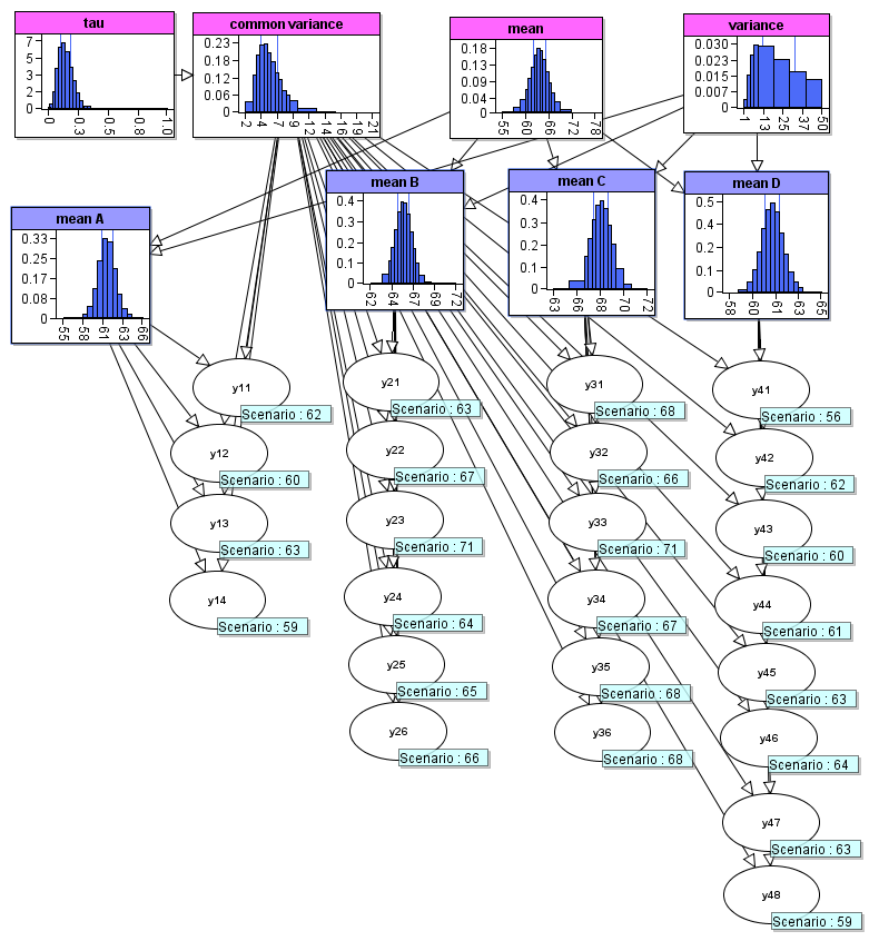
asia_model$to_cmpx()This is a BN which uses experiment observations to estimate the parameters of a distribution. In the model structure, there are nodes for the parameters which are the underlying parameters for all the experiments and the observed values inform us about the values for these parameters. The model in agena.ai Modeller is given below:
In this section we will create this model entirely in RAgena environment. We can start with creating first four nodes.
Mean and variance nodes:
library(agena.ai)

#First we create the "mean" and "variance" nodes

mean <- new("Node", id = "mean", simulated = TRUE)
mean$set_expressions("Normal(0.0,100000.0)")

variance <- new("Node", id = "variance", simulated = TRUE)
variance$set_expressions("Uniform(0.0,50.0)")
Common variance and tau nodes:
#Now we create the "common variance" and its "tau" parameter nodes

tau <- new("Node", id = "tau", simulated = TRUE)
tau$set_expressions("Gamma(0.001,1000.0)")

common_var <- new("Node", id = "common_var", name = "common variance", simulated = TRUE)
common_var$add_parent(tau)
common_var$set_expressions("Arithmetic(1.0/tau)")
Now we can create the four mean nodes, using a for loop and list of Nodes:
#Creating a list of four mean nodes, "mean A", "mean B", "mean C", and "mean D"

mean_names <- c("A", "B", "C", "D")
means_list <- vector(mode = "list", length = length(mean_names))

for (i in seq_along(mean_names)) {
  node_id <- paste0("mean",mean_names[i])
  node_name <- paste("mean",mean_names[[i]])
  means_list[[i]] <- new("Node", id = node_id, name = node_name, simulated = TRUE)
  means_list[[i]]$add_parent(mean)
  means_list[[i]]$add_parent(variance)
  means_list[[i]]$set_expressions("Normal(mean,variance)")
}
Now we can create the experiment nodes, based on the number of observations which will be entered:
# Defining the list of observations for the experiment nodes
# and creating the experiment nodes y11, y12, ..., y47, y48

observations <- list(c(62, 60, 63, 59),
                     c(63, 67, 71, 64, 65, 66),
                     c(68, 66, 71, 67, 68, 68),
                     c(56, 62, 60, 61, 63, 64, 63, 59))

obs_nodes_list <- vector(mode = "list", length = length(mean_names))
for (i in seq_along(obs_nodes_list)) {
  obs_nodes_list[[i]] <- vector(mode = "list", length = length(observations[[i]]))
  this_mean_id <- means_list[[i]]$id

  for (j in seq_along(obs_nodes_list[[i]])) {
    node_id <- paste0("y",i,j)
    obs_nodes_list[[i]][[j]] <- new("Node", id = node_id, simulated = TRUE)
    obs_nodes_list[[i]][[j]]$add_parent(common_var)
    obs_nodes_list[[i]][[j]]$add_parent(means_list[[i]])
    this_expression <- paste0("Normal(",this_mean_id,",common_var)")
    obs_nodes_list[[i]][[j]]$set_expressions(this_expression)
  }
}
We can create a network for all the nodes:
#Creating the network for all the nodes

diet_network <- new("Network", id = "Hierarchical_Normal_Model_1",
                            name = "Hierarchical Normal Model")
And add all the nodes to this network. First eight nodes:
# Adding first eight nodes to the network

for (nd in c(mean, variance, tau, common_var, means_list)) {
  diet_network$add_node(nd)
}
Then adding all the experiment nodes:
# Adding all the experiment nodes to the network

for (nds in obs_nodes_list) {
  for (nd in nds) {
    diet_network$add_node(nd)
  }
}
Now we can create a model with this network:
# Creating a model with the network

diet_model <- new("Model", networks = list(diet_network),
                        id = "Diet_Experiment_Model")
We enter all the observation values to the nodes:
# Entering all the observations

for (i in seq_along(observations)) {
  for (j in seq_along(observations[[i]])) {
    this_node_id <- paste0("y",i,j)
    this_value <- observations[[i]][j]
    diet_model$enter_observation(node = this_node_id,
                                 network = diet_model$networks[[1]]$id,
                                 value = this_value)
  }
}
Now the model is ready with all the information, we can export it to either a .json or a .cmpx file for agena.ai calculations, either locally or on Cloud:
# Creating json or cmpx file for the model
diet_model$to_json()
diet_model$to_cmpx()