ferrn

The ferrn package extracts key components from the data object collected during projection pursuit (PP) guided tour optimisation, produces diagnostic plots, and calculates PP index scores.

Installation

You can install the development version of ferrn from GitHub with:

# install.packages("remotes")
remotes::install_github("huizezhang-sherry/ferrn")

Visualise PP optimisation

The data object collected during a PP optimisation can be obtained by assigning the tourr::annimate_xx() function a name. In the following example, the projection pursuit is finding the best projection basis that can detect multi-modality for the boa5 dataset using the holes() index function and the optimiser search_better:

set.seed(123456)
holes_1d_better <- animate_dist(
  ferrn::boa5,
  tour_path = guided_tour(holes(), d = 1, search_f =  search_better), 
  rescale = FALSE)
holes_1d_better

The data structure includes the basis sampled by the optimiser, their corresponding index values (index_val), an information tag explaining the optimisation states, and the optimisation method used (search_better). The variables tries and loop describe the number of iterations and samples in the optimisation process, respectively. The variable id serves as the global identifier.

The best projection basis can be extracted via

library(ferrn)
library(dplyr)
holes_1d_better %>% get_best()
#> # A tibble: 1 × 8
#>   basis         index_val info          method        alpha tries  loop    id
#>   <list>            <dbl> <chr>         <chr>         <dbl> <dbl> <dbl> <int>
#> 1 <dbl [5 × 1]>     0.914 interpolation search_better    NA     5     6    55
holes_1d_better %>% get_best() %>% pull(basis) %>% .[[1]]
#>              [,1]
#> [1,]  0.005468276
#> [2,]  0.990167039
#> [3,] -0.054198426
#> [4,]  0.088415793
#> [5,]  0.093725721
holes_1d_better %>% get_best() %>% pull(index_val)
#> [1] 0.9136095

The trace plot can be used to view the optimisation progression:

holes_1d_better %>% 
  explore_trace_interp() + 
  scale_color_continuous_botanical()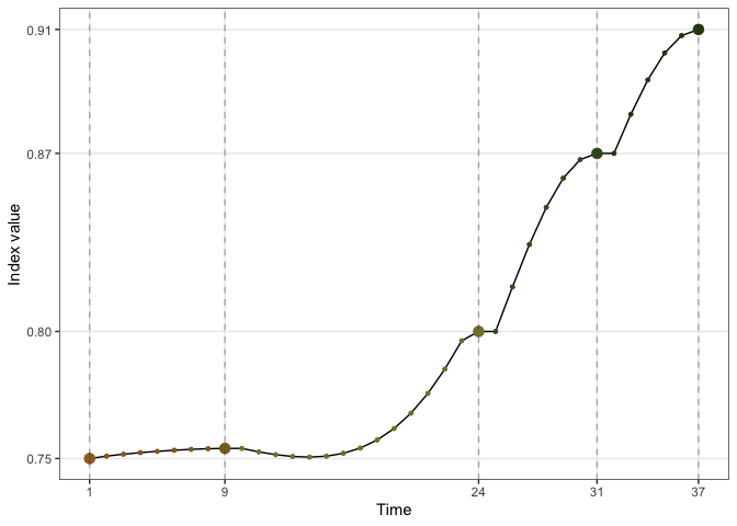

Different optimisers can be compared by plotting their projection bases on the reduced PCA space. Here holes_1d_geo is the data obtained from the same PP problem as holes_1d_better introduced above, but with a search_geodesic optimiser. The 5 \(\times\) 1 bases from the two datasets are first reduced to 2D via PCA, and then plotted to the PCA space. (PP bases are ortho-normal and the space for \(n \times 1\) bases is an \(n\)-d sphere, hence a circle when projected into 2D.)

bind_rows(holes_1d_geo, holes_1d_better) %>%
  bind_theoretical(matrix(c(0, 1, 0, 0, 0), nrow = 5),
                   index = tourr::holes(), raw_data = boa5) %>% 
  explore_space_pca(group = method, details = TRUE)  +
  scale_color_discrete_botanical()

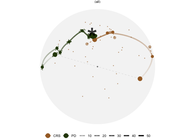
The same set of bases can be visualised in the original 5-D space via tour animation:

bind_rows(holes_1d_geo, holes_1d_better) %>%
  explore_space_tour(flip = TRUE, group = method,
                     palette = botanical_palettes$fern[c(1, 6)],
                     max_frames = 20, 
                     point_size = 2, end_size = 5)

Reference